


Neural networks is a subset of machine learning. They are extremely versatile and powerful, with applications ranging from computer vision to language models.
Python has some very powerful libraries for neural networks, one of which is Keras.

However, in this post we will explore the basic functionality of neural networks using Numpy only. We will train a model to classify types of irises based on their petal dimensions. You can download the dataset from Kaggle.
Structure of Neural Networks
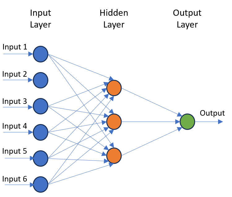
A neural network is a model that predicts an output based on a given input. The name of the model derives from its structure. Like the brain, artificial neural networks consists of a multitude of interconnected neurons, which it organizes into layers with a minimum of 3 distinct layers:
- Input layer: This is where the known data is fed into the model. The number of neurons is equal to the number of inputs.
- Hidden layers: These layers determines patterns that links the input data to the output data. The network can have one or more hidden layers.
- Output layer: This layer gives the prediction of the network. The number of neurons in this layer is equal to the number of values that the model predicts.
What is a neuron?
A neuron takes a bunch on inputs, calculates a weighted sum of these inputs, adds a bias and then returns an output value based on an activation function.
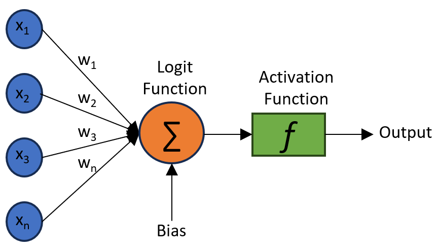
The weights represent the strength between strength between the layers. The higher the weight, the higher the impact of the input on the output. The neural network adjust these weights during training to minimize the difference between the predicted output and the actual output.
The biases are added to each neuron to account for situatons where all the inputs have zero or low values. They help the model to capture the overall trend of the data. Similar to the weights, the biases are also learned during training.
The activation functions introduce non-linearities to the model. They activate/deactivate a neuron based on the weighted sum of all its inputs and biases. Without them, the model will just be a linear regression model. The activation functions help the model to learn complex patterns and relations in the data. Below is a list of common activation functions.
Common activation functions for Neural Networks
| Function | \bf f(x) | \bf f'(x) | |
|---|---|---|---|
| Linear | x | 1 | |
| Binary step | \begin{cases} 0 & \text{if } x < 0 \\ 1 &\text{if } x\ge0 \end{cases} | \begin{cases} 0 & \text{if } x \ne 0 \\ ? &\text{if } x=0 \end{cases} | |
| Sigmoid | \frac{1}{1 + e^{-x}} | f(x)(1-f(x)) | |
| Hyperbolic Tanget (tanh) | \frac{e^{2x}-1}{e^{2x}+1} | 1 – f(x)^2 | |
| ArcTan | tan^{-1}(x) | \frac{1}{x^2+1} | |
| Rectified Linear Unit (ReLU) | \begin{cases} 0 & \text{if } x < 0 \\ x &\text{if } x\ge0 \end{cases} | \begin{cases} 0 & \text{if } x < 0 \\ 1 &\text{if } x\ge0 \end{cases} | |
| Parametric Rectified Linear Unit (PReLU) | \begin{cases} ax & \text{if } x < 0 \\ x &\text{if } x\ge0 \end{cases} | \begin{cases} a & \text{if } x < 0 \\ 1 &\text{if } x\ge0 \end{cases} | |
| Exponential Linear Unit (ELU) | \begin{cases} a(e^x-1) & \text{if } x < 0 \\ x &\text{if } x\ge0 \end{cases} | \begin{cases} f(x) + a & \text{if } x < 0 \\ 1 &\text{if } x\ge0 \end{cases} | |
| Softplus | log_e(1+e^x) | \frac{1}{1 + e^{-x}} |
Numpy Implementation
The activations functions that will be used by this model are stored in a dictionary.
import numpy as np

activation_functions = dict(
    relu = lambda X: np.maximum(0, X),
    softmax = lambda X: np.exp(X) / np.exp(X).sum(axis = 1, keepdims = True)
)
Define the architecture of the Neural Network
We will keep it simple, with only 2 dense layers. A dense layer is a type where each neuron is connected to each neuron of the preceding layer.
def dense_layer(neurons, activation = 'relu'):
    """
    Defines the forward and backward pass functions for a dense layer.
        - neurons: number of neurons in the layer.
        - activation: name of activation function to be used.
    """
    def forward(inputs, weights, bias):
        """
        Calculates the outputs of the logit and activation functions
        for each neuron.
        """
        Z_curr = inputs.dot(weights.T) + bias
        A_curr = activation_functions[activation](Z_curr)
        return A_curr, Z_curr

    def backward(dA_curr, W_curr, Z_curr, A_prev):
        """
        Calculates the gradients of the predictions, weights and biases.
            dA_curr: gradient of the current predictions.
            W_curr: current weights of the layer.
            Z_curr: current logit function output.
            A_prev: previous activation function output.
        """
        if activation == 'softmax':
            dW = A_prev.T.dot(dA_curr)
            db = dA_curr.sum(axis=0, keepdims=True)
            dA = dA_curr.dot(W_curr)
        else:
            dZ = relu_derivative(dA_curr, Z_curr)
            dW = A_prev.T.dot(dZ)
            db = dZ.sum(axis=0, keepdims=True)
            dA = dZ.dot(W_curr)
        return dA, dW, db

    return dict(forward = forward, backward = backward, neurons = neurons)
The next step is to initialize each of the layers. All this step does is assign the activation function to each layer, as specified in the previous step.
def init_architecture(layers, X_train):
    for i, layer in enumerate(layers):
        layer['input_dim'] = layers[i - 1]['neurons'] if i > 0 \
        else X_train.shape[1]
        layer['output_dim'] = layer['neurons']

init_architecture(layers, X_train)
The final step in setting up the model is to initialize the weights and biases.
def init_weights(layers, debug = False):
    from numpy import random, zeros
    params = []
    if debug:
        random.seed(99)
    for layer in layers:
        params.append(dict(
            W = random.uniform(
                low = -1,
                high = 1,
                size = (layer['output_dim'], layer['input_dim'])
            ),
            b = zeros((1, layer['output_dim'])),
        ))
    return params
Training the Neural Network
The neural network model is trained by iterating through the following 5 steps:
- Forward propagation
- Calculate accuracy
- Calculate loss
- Backwards propagation
- Update weights and biases
Forward propagation
Forward propagation is a step during the training of a neural network. It is simply the process where the input data is fed through the neural network to produce predictions on the output (moving left to right in Figure 1).
For each neuron, the model multiplies the input data by the weights then adds the biases. The result is then passed on to the connected neurons in the next layer. The process is repeated until the final output is obtained.
def forward_propagation(layers, A_curr, params, memory):
    """
    Calls the forward pass function for each layer.
        - A_curr: output of the activation function.
        - params: list with weights and biases for each layer
        - memory: list with the previous activation function output
                  and current logit function output.
    """
    for i in range(len(params)):
        A_prev = A_curr.copy()
        A_curr, Z_curr = layers[i]['forward'](
            A_prev,
            params[i]['W'],
            params[i]['b']
        )
        memory.append(dict(inputs = A_prev, Z = Z_curr))
    return A_curr
Calculate accuracy and loss
After obtaining the predictions, the model calculates the difference between the predicted output and actual target. The loss represents how far off the predictions are from the true values.
def calculate_accuracy(predicted, actual):
    """
    Calculate accuracy after each iteration
    """
    return (predicted.argmax(axis = 1) == actual).mean()

def calculate_loss(predicted, actual):
    """
    Calculates the cross-entropy loss.
    """
    from numpy import log
    n = len(actual)
    loss = -log(predicted[range(n), actual]).sum() / n
    return loss
Backwards propagation
Backward propagation updates the model’s weights and biases to minimize the loss. During backwards propagation, the model calculates the gradient of the loss with respect to each parameter in the network. The model then updates the weights and biases in the opposite direction of the gradient, with the goal of minimizing the loss. Optimization algorithms like stochastic gradient descent (SGD) or variants like Adam are used to minimize the loss.
def backwards_propagation(layers, predicted, actual, gradients):
    n = len(actual)

    # compute the gradient on predictions
    dS = predicted
    dS[range(n), actual] -= 1
    dS /= n
    dA_prev = dS

    n = len(layers)
    for i in range(n):
        i = n - 1 - i
        dA_curr = dA_prev

        A_prev = memory[i]['inputs']
        Z_curr = memory[i]['Z']
        W_curr = params[i]['W']

        dA_prev, dW_curr, db_curr = layers[i]['backward'](
            dA_curr,
            W_curr,
            Z_curr,
            A_prev
        )
        gradients.append(dict(dW = dW_curr, db = db_curr))
Update the weights and biases
The final step in the training loop is to update the weights and biases. This is done be deducting the product of the gradient and learning rate from the current values.
def update(params, gradients, lr=0.01):
    """
    Update the model parameters --> lr * gradient
    """
    n = len(gradients)
    for i in range(len(params)):
        params[i]['W'] -= lr * gradients[n - 1 - i]['dW'].T
        params[i]['b'] -= lr * gradients[n - 1 - i]['db']
Training the Neural Network
def model(X_train, y_train, layers, epochs = 25, debug = False):
    memory = []
    accuracy = []
    loss = []
    gradients = []
    lr = 0.01

    init_architecture(layers, X_train)
    params = init_weights(layers, debug = debug)
    for i in range(epochs):
        yhat = forward_propagation(layers, X_train, params, memory)
        accuracy.append(calculate_accuracy(yhat, y_train))
        loss.append(calculate_loss(yhat, y_train))
        backwards_propagation(layers, yhat, y_train, gradients)
        update(params, gradients, lr = lr)

    def predict(X):
        yhat = forward_propagation(
            architecture,
            X,
            params,
            memory
        ).argmax(axis = 1)
        return yhat
    return predict, accuracy, loss

layers = [
    dense_layer(neurons = 6, activation = 'relu'),
    dense_layer(neurons = 3, activation = 'softmax'),
]

def get_data(path):
    from numpy import array
    data = read_csv(path, index_col=0)
    cols = list(data.columns)
    target = cols.pop()
    X = data[cols].copy()
    y = data[target].copy()
    y = LabelEncoder().fit_transform(y)
    return array(X), array(y)
X, y = get_data(r"C:\Users\mechanicalcoder\Downloads\archive\Iris.csv")

predict, accuracy, loss = model(X.copy(), y.copy(), layers)
Keras Implementation
from keras.models import Sequential
from keras.layers import Dense
import tensorflow as tf
from tensorflow.keras.optimizers import SGD

yc = tf.keras.utils.to_categorical(y, num_classes=3)

model = Sequential()
model.add(Dense(6, activation='relu'))
model.add(Dense(3, activation='softmax'))
model.compile(
    SGD(learning_rate=0.01),
    loss='categorical_crossentropy',
    metrics=['accuracy']
)
hist = model.fit(x = X, y = yc, epochs = 25)
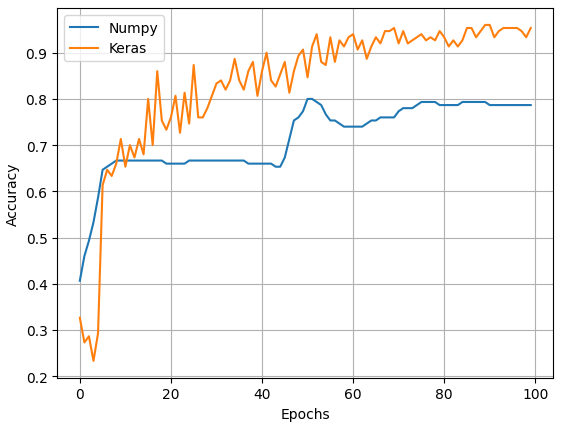
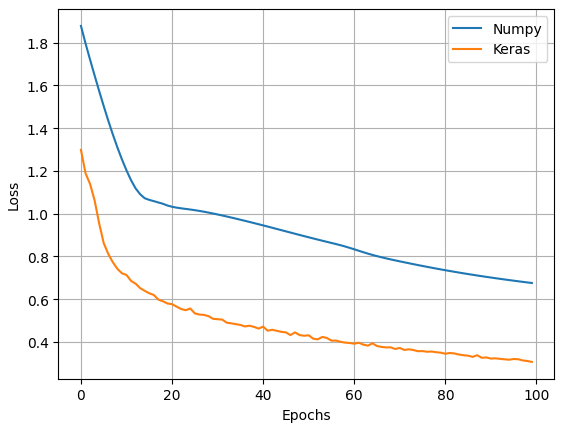
Comparing the Neural Networks
The two plots below compare the Numpy and Keras models in terms of accuracy and loss. Figure 4 can be improved by adding the validated loss thus monitoring overfitting. It is clear that the keras model is clearly better. However, the goal of this exercise was not to beat Keras but to understand the basics of Neural Networks.
Conclusion
Breaking the Neural Network down into its building blocs helps to understand it better. As a result you will be able to perform hyperparameter tuning better, thus building better models.
In a following post we will delve into ways to improve the Numpy model and see how it performs with time series forecasting.