In today’s fast-paced and data-driven world, accurate predictions are key. One powerful tool for achieving this is LSTM networks, which have been widely used for Time Series Forecasting. In this blog, we’ll delve into the concept of Time Series Forecasting with LSTM. So, buckle up and get ready to explore the exciting world of Time Series Forecasting with LSTM!

What is LSTM?

LSTM stand for Long Short-Term Memory. It is a type of Recurrent Neural Network (RNN) which processes sequential data. It was developed to address a problem in traditional RNNs: vanishing gradients.

Why the gradient is necessary in Time Series Forecasting

The gradient is the derivative of the loss function. It is derived with respect to the weights which reduces the loss of the cost function. The gradient influence the adjustment of the weights. Therefore, it is important to correctly determine the gradient throughout the learning period.

Vanishing gradients is an occurrence where the gradient signal becomes very weak with time. In RNNs, the gradient backpropagates through many time steps. As a result the gradient becomes smaller with each time step. The smaller the gradient gets, the less its impact on the weights gets. Therefore, it will reach a point where the loss is no longer reducing.

In deep RNNs the problem is even more pronounced, where the gradients passes through multiple layers. This leads to almost no update of the weights. It can result in the model not being able to learn from the input data and produce accurate predictions.

How LSTMs accurately perform Time Series Forecasting

LSTMs overcome the vanishing gradient problem by using memory cells, which can store information for long periods of time. Gates control the flow of information. Not only in and out of cells, but also the output of the model. These components allow the LSTM to selectively preserve or forget information and to make use of past information to make predictions based on the current input.

LSTMs have proven to be extremely effective. A few examples include:

• speech recognition
• image generation
• natural language processing
• time series forecasting

Preparing the training data

Generating data to play with

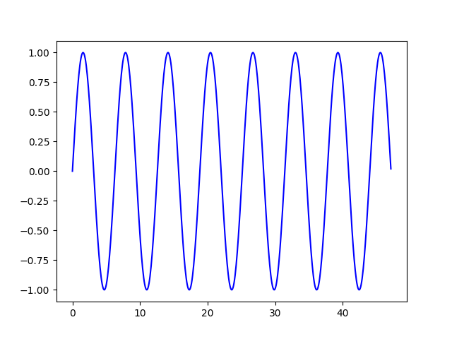
To keep things simple we will predict a sine wave. We will use a range of timesteps to train our model and then predict the next few timestep. Below is an example of a sine wave, where x will be the input data and y the output data.

import numpy as np
x = np.linspace(0, 8 * np.pi, 500).reshape(-1,1)
y = np.sin(x).reshape(-1,1)

Before we can use the data, we need to process the data. The shape of the training data is very important.

The input data for Time Series Forecasting

The training data will consist of 2 datasets: input data and output data.

The input data is a sequence of numerical values that represent some kind of time-series data such as stock prices, weather data, speech signals, etc. The length of the input sequence is a hyperparameter of the model which determines the memory capacity of the LSTM network.

The output data is a prediction or a class label based on the input sequence. The LSTM model takes a sequence of past values as input then predicts the next value in the sequence. In a classification problem, the LSTM takes a sequence of values as input and outputs a class label. The output can be a single value or a probability distribution over multiple classes.

With the Time Series Forecasting of a sine wave, the input data will be the x values and the output data the y values. However, before it can be fed into the model, we need to process the data. The shape of the input data is (number of samples, timestamps, features) while for the output data it is (number of samples, features)

For example: there are 100 samples, each consisting of 10 timesteps (10 x values) with 1 feature (the x value). The shape of the input array would then be (100, 10, 1) . On the other hand the shape of the output array would be (100, 1).

Creating a windowed dataset

A windowed dataset consists of overlapping windows of time steps. It provides the LSTM model with a sequence of previous time steps to use as input to make predictions for the next time step.

For example, let us take a a time series with 100 time steps. You can create windows of size 10 that overlap by 9 time steps. This way, you have 10 windows, each containing the previous 10 time steps, and you can use the first 9 time steps in each window as input to make predictions for the 10th time step.

LSTM networks process sequences of input data and make predictions based on the input sequence. Therefore, windowed datasets are necessary to train the LSTM model. By creating windows of previous time steps, you are providing the LSTM model with a sequence of input data that it can use to make predictions for the next time step.

Creating a windowed dataset also helps to overcome the issue of vanishing gradients in LSTMs. This is because the LSTM model traines to make predictions based on a short sequence of input data, which makes it easier for the gradients to propagate through the network during training.

x_train = []
y_train = []
for i in range(len(y) - lookback - forecast + 1):
    x_sample = x[i:i + lookback]
    x_train.append(x_sample)
    y_sample = y[i + lookback:i + lookback + forecast, 0]
    y_train.append(y_sample)

x_train = np.array(x_train)
y_train = np.array(y_train)

The parameters of the window

The lookback variable determines the size of the windows in the x_train array. The x_train array consists of overlapping windows of past time steps, where each window has a size equal to the lookback value. The first window will start at the first time step, and subsequent windows will start lookback time steps apart.

The forecast variable determines the size of the target array, y_train. Each window in the x_train array paires with a target value, y_train.

For example, let lookback=10 and forecast=1. Each window in the x_train array consists of the past 10 time steps while the target value, y_train, is 1 time step in the future.

The makeup of the Time Series Forecasting model

The time series we will forecast will be a sine wave. Therefore, the model will be very smple. The Keras library provides a Sequential model, which can create a LSTM model. The Sequential model is a linear stack of layers, where you can simply add one layer at a time. The code to build a simple LSTM model using the Sequential model in Keras is as follows:

from keras.models import Sequential
from keras.layers import Dense, LSTM

model = Sequential()
model.add(LSTM(UNITS, input_shape=(LOOKBACK, FEATURES)))
model.add(Dense(FORECAST))

Sequential is the simplest and most common type of model in Keras, which consists of a linear stack of layers. It uses a single input to produce a single output. In the example the Sequential layer consists of 2 layers: a LSTM layer and a Dense layer.

Number of neurons

The number of units in an LSTM layer represents the dimensionality of the output space. That is the number of neurons or nodes in the layer. In other words, the number of units determines the capacity of the layer to capture patterns and make predictions.

In the context of time series forecasting, each unit in an LSTM layer is like a parallel processing element. Each unit is able to learn and extract information from the input sequence. It uses its internal memory cell, input gate, forget gate, and output gate to process the input sequence and generate its own representation of the input.

In general, the number of units in an LSTM layer depends on the complexity of the input data and the desired capacity of the model. A larger number of units will allow the model to capture more complex patterns in the data, but will also increase the risk of overfitting. On the other hand, a smaller number of units will result in a simpler model with a lower capacity to capture complex patterns in the data. The optimal number of units can be determined through experimentation. This is done by testing the model on a validation set and selecting the number of units that gives the best performance.

The input shape

The input shape argument in the first layer of a Keras model typically consists of two values: the number of time steps and the number of features. The number of time steps represents the number of time steps in a single sample while the number of features represents the number of variables in each time step.

For example, in the case of a univariate time series forecasting problem, where you want to predict the next value in a sequence given the previous n values, the input shape would be (n, 1), where n is the number of time steps and 1 is the number of features (the single time series value).

In the case of a multivariate time series forecasting problem, where you want to predict the next value in a sequence given the previous n values and other variables, the input shape would be (n, m), where n is the number of time steps and m is the number of features (the m variables).

The dense layer

The Dense layer in a neural network is a fully connected layer, which means that each neuron in the layer is connected to every neuron in the previous layer. The Dense layer implements a linear operation on its inputs, where each input is multiplied by a weight and then added to a bias term.

In a neural network for time series forecasting, the output layer is typically a Dense layer, which makes the final prediction. The number of neurons in the output layer will depend on the number of variables you are trying to predict. For example, in the case of univariate time series forecasting, the output layer will have one neuron, since you are trying to predict a single value. In the case of multivariate time series forecasting, the output layer will have m neurons, where m is the number of variables you are trying to predict.

Compiling the Time Series Forecasting model

The compilation step configures the model for training. It is therefore a necessary step before training. It involves specifying the loss function, the optimizer, and any metrics.

The loss function measures the difference between the predicted output and the true target values during training. The optimizer then updates the model weights based on the gradients calculated from the loss function. The optimizer is responsible for minimizing the loss function to improve the model’s predictions.

The metrics evaluate the performance of the model on a validation or test set. Common metrics for time series prediction include mean squared error (MSE) and mean absolute error (MAE).

By compiling the model, you are defining the optimization problem that the model will solve during training. This allows the model to use the specified loss function, optimizer, and metrics during the training process to improve its predictions.

model.compile(loss='mean_squared_error', optimizer='adam')

Fitting the model

Fitting a model in machine learning means training the model on a given dataset. The goal of fitting is to optimize the model’s parameters to minimize the difference between the model’s predictions and the actual target values in the training dataset.

Fitting a model involves training the model on a training dataset, where the model’s weights updates iteratively based on the gradients calculated from the loss function. The loss function measures the difference between the model’s predictions and the actual target values in the training dataset. The optimization process continues until a specified number of epochs or until the change in the loss function is below a certain threshold.

The “fit” method in the machine learning library is fits the model to the training data. It requires the training data (X_train and y_train), the number of epochs to train the model, the batch size to use during training, and any other relevant parameters. During training, the model will make predictions on the training data, calculate the loss, and update the model’s weights to minimize the loss.

Fitting the model is a crucial step in the machine learning process, as it trains the model on the given dataset and creates a model that is ready to make predictions on new unseen data.

hist = model.fit(x_train, y_train, epochs=100, batch_size=32, verbose=0)

The number of epochs

The “epochs” argument in a machine learning model is the number of complete iterations over the entire training dataset. An epoch is one pass through the entire training dataset, where each sample in the training dataset is used once for updating the model parameters.

The training process involves updating the model weights iteratively based on the gradient of the loss function. During each iteration, a batch of samples from the training dataset is used to calculate the gradient. The model weights then updates accordingly. The number of iterations it takes to go through the entire training dataset once is one epoch.

The epochs argument in the training process allows you to specify the number of complete passes through the training dataset that the model should make during training. The larger the number of epochs, the more the model is training. Therefore, it has to improve its accuracy. However, too many epochs can lead to overfitting, where the model starts to memorize the training data and becomes less able to generalize to new unseen data. It is therefore important to choose a suitable number of epochs that balances the model’s ability to learn from the training data and avoid overfitting.

The size of the batch

The batch size argument in the fit method of a Keras model specifies the number of samples to use in one forward/backward pass. The value of batch_size can be any positive integer, but it is common to use values between 32 and 128.

The choice of batch size depends on the size of your data and the amount of memory available on your GPU or CPU. A larger batch size requires more memory, while a smaller batch size requires more iterations to reach convergence.

For example, if you have a training set of 100 samples, you can choose a batch size of 10, 20, or 50. The model will update its weights after each batch, and it will need 10, 5, or 2 forward/backward passes to process the entire training set.

Time Series Forecasting

To use the LSTM model to predict the next time step, you need to provide the model with the previous time steps as input. You can use the predict method of the model to get the predicted values for the next time step.

Here’s an example of how to make a prediction for the next time step:

# reshape the input data to have the correct shape for the LSTM model
input_data = np.array(x[:LOOKBACK]).reshape(1, LOOKBACK, FEATURES)

# make the prediction
prediction = model.predict(input_data)

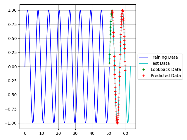
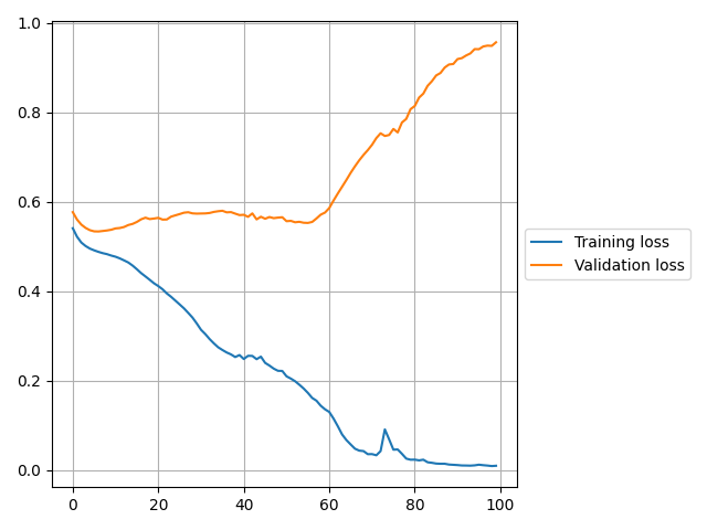
Figures 3 and 4 below shows the results of the predictions. The first figure used the training data to make the predictions, while the second figure used the test data. Predicting the training data proved very accurate, however the test data not so much. This variation can be explained by Figure 4.

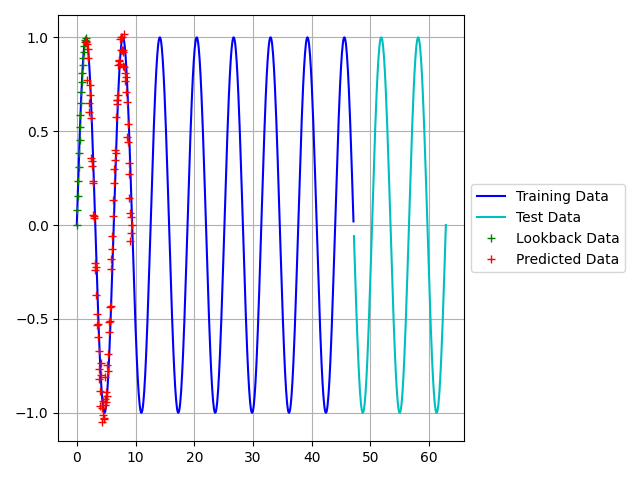
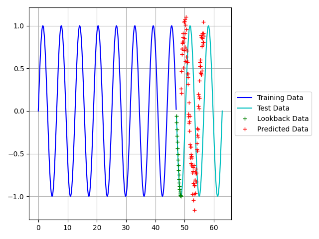
The training loss is far less than the validation loss, which is an indication of overtraining. The purpose of this post was to first form an understanding of LSTM models. Therefore, we will not delve into the optimization of the model yet. However, optimization of this model is discussed HERE.

Conclusion

In conclusion, LSTM networks have proven to be a powerful tool for performing Time Series Forecasting. By incorporating memory and feedback mechanisms, LSTMs are able to capture long-term dependencies in sequential data and make accurate predictions. The flexibility and ease of use of LSTMs in Python, combined with its ability to handle large and complex data, make it a popular choice for Time Series Forecasting tasks. Whether you are a beginner or an experienced data scientist, LSTMs provide a great starting point for developing robust and effective time series forecasting models. By mastering the use of LSTMs, you will be well-equipped to tackle a wide range of time-sensitive data-driven problems with confidence and success.